The libr package brings the concepts of data libraries, data dictionaries, and data steps to R.
- A data library is an object used to define and
manage an entire directory of data files.
- A data dictionary is a data frame full of information about a data library, data frame, or tibble.
- A data step is a mechanism to perform row-by-row processing of data.
These concepts have been available in SAS® software for decades. But they have not been available in R … until now!
The libr package also includes an enhanced equality operator to make data comparisons more intuitive.
Key Functions
The above concepts are implemented in the libr package with four key functions. They are:
-
libname(): Creates a data library -
dictionary(): Creates a data dictionary -
datastep(): Performs row-by-row processing of data
How to Use
Let’s look at some simple examples of each of the four functions above. These examples will be using some sample data. The sample data is included in the libr package, and also available for download here.
The libname() Function
The libr libname() function is quite
similar to the SAS® libname statement. The first parameter
is the name of the library. The second parameter is a path to a
directory the library will point to. The third parameter is the engine
with which to read and write the data.
library(libr)

# Get path to sample data
pkg <- system.file("extdata", package = "libr")

# Define data library
libname(sdtm, pkg, "csv")
The libname() function above will send two types of
information to the console:
- The column specifications for each data file imported
- A summary print-out of the library
The summary print-out looks like this:
# library 'sdtm': 8 items
- attributes: csv not loaded
- path: C:/packages/libr/inst/extdata
- items:
  Name Extension Rows Cols     Size        LastModified
1   AE       csv  150   27  88.1 Kb 2020-09-18 14:30:23
2   DA       csv 3587   18 527.8 Kb 2020-09-18 14:30:23
3   DM       csv   87   24  45.1 Kb 2020-09-18 14:30:23
4   DS       csv  174    9  33.7 Kb 2020-09-18 14:30:23
5   EX       csv   84   11    26 Kb 2020-09-18 14:30:23
6   IE       csv    2   14    13 Kb 2020-09-18 14:30:23
7   SV       csv  685   10  69.9 Kb 2020-09-18 14:30:24
8   VS       csv 3358   17   467 Kb 2020-09-18 14:30:24
The summary displays what type of library it is, where it is located, and what data (if any) is already in the library directory. In this case, there are eight ‘csv’ files available.
For each of the eight files, the libname() function also
displayed the column specifications used to import the data file. A
column specification looks like this:
$VS

-- Column specification ------------------------------------------
cols(
  STUDYID = col_character(),
  DOMAIN = col_character(),
  USUBJID = col_character(),
  VSSEQ = col_double(),
  VSTESTCD = col_character(),
  VSTEST = col_character(),
  VSPOS = col_character(),
  VSORRES = col_double(),
  VSORRESU = col_character(),
  VSSTRESC = col_double(),
  VSSTRESN = col_double(),
  VSSTRESU = col_character(),
  VSBLFL = col_character(),
  VISITNUM = col_double(),
  VISIT = col_character(),
  VSDTC = col_date(format = ""),
  VSDY = col_double()
)
The column specification shows how the data was imported. Since ‘csv’
files do not contain well-defined data type information on each of the
columns, the libname() function has to guess at the data
types. The column specification shows you what the guesses were. This is
useful information. You should review these column specifications to see
if the libname() function guessed correctly. If it did not
guess correctly, you can control the import data types by sending a
specs() collection of import_spec() objects to
the import_specs parameter on the libname()
function. See the specs() documentation for an example and
additional details.
Accessing Data
Observe that there is difference between the SAS®
libname statement and the libr
libname() function. The difference is that after the SAS®
libname statement is called, the data is immediately
available to your code using two-level (<library>.<dataset>)
syntax.
With the libr function, on the other hand, the data is immediately available using list syntax on the library variable name. That means you can get to your data using the dollar sign ($), like this:
# View a dataset
sdtm$DM
# # A tibble: 87 × 24
#    STUDYID DOMAIN USUBJID SUBJID RFSTDTC    RFENDTC RFXSTDTC RFXENDTC RFICDTC    RFPENDTC
#    <chr>   <chr>  <chr>   <chr>  <date>     <date>  <lgl>    <lgl>    <date>     <date>
#  1 ABC     DM     ABC-01… 049    2006-11-07 NA      NA       NA       2006-10-25 NA
#  2 ABC     DM     ABC-01… 050    2006-11-02 NA      NA       NA       2006-10-25 NA
#  3 ABC     DM     ABC-01… 051    2006-11-02 NA      NA       NA       2006-10-25 NA
#  4 ABC     DM     ABC-01… 052    2006-11-06 NA      NA       NA       2006-10-31 NA
#  5 ABC     DM     ABC-01… 053    2006-11-08 NA      NA       NA       2006-11-01 NA
#  6 ABC     DM     ABC-01… 054    2006-11-16 NA      NA       NA       2006-11-07 NA
#  7 ABC     DM     ABC-01… 055    2006-12-06 NA      NA       NA       2006-10-31 NA
#  8 ABC     DM     ABC-01… 056    2006-11-28 NA      NA       NA       2006-11-21 NA
#  9 ABC     DM     ABC-01… 113    2006-12-05 NA      NA       NA       2006-11-28 NA
# 10 ABC     DM     ABC-01… 114    2006-12-14 NA      NA       NA       2006-12-01 NA
# #  77 more rows
# #  14 more variables: DTHDTC <lgl>, DTHFL <lgl>, SITEID <chr>, BRTHDTC <date>, AGE <dbl>,
# #   AGEU <chr>, SEX <chr>, RACE <chr>, ETHNIC <chr>, ARMCD <chr>, ARM <chr>, ACTARMCD <lgl>,
# #   ACTARM <lgl>, COUNTRY <lgl>
# #  Use `print(n = ...)` to see more rows
Using this syntax, your dataset can be passed into any R function. For example, here we can subset the dataset for a particular subject:
# Subset the data
dat <- subset(sdtm$DM, SUBJID == '050')

# View results
dat
# # A tibble: 1 × 24
#   STUDYID DOMAIN USUBJID  SUBJID RFSTDTC    RFENDTC RFXSTDTC RFXENDTC RFICDTC    RFPENDTC
#   <chr>   <chr>  <chr>    <chr>  <date>     <date>  <lgl>    <lgl>    <date>     <date>
# 1 ABC     DM     ABC-01-… 050    2006-11-02 NA      NA       NA       2006-10-25 NA
# #   14 more variables: DTHDTC <lgl>, DTHFL <lgl>, SITEID <chr>, BRTHDTC <date>, AGE <dbl>,
# #   AGEU <chr>, SEX <chr>, RACE <chr>, ETHNIC <chr>, ARMCD <chr>, ARM <chr>, ACTARMCD <lgl>,
# #   ACTARM <lgl>, COUNTRY <lgl>
The dollar sign syntax shown above is recommended for the most memory-efficient programming. If you are writing production code to be run in batch, use the dollar sign syntax.
The lib_load() Function
For convenience, the package also provides a way to get two-level dot
syntax, similar to SAS®. To get the dot syntax, you first have to call
the lib_load() function.
lib_load(sdtm)
# # library 'sdtm': 8 items
# - attributes: csv loaded
# - path: C:/packages/libr/inst/extdata
# - items:
#   Name Extension Rows Cols     Size        LastModified
# 1   AE       csv  150   27  88.1 Kb 2020-09-18 14:30:23
# 2   DA       csv 3587   18 527.8 Kb 2020-09-18 14:30:23
# 3   DM       csv   87   24  45.1 Kb 2020-09-18 14:30:23
# 4   DS       csv  174    9  33.7 Kb 2020-09-18 14:30:23
# 5   EX       csv   84   11    26 Kb 2020-09-18 14:30:23
# 6   IE       csv    2   14    13 Kb 2020-09-18 14:30:23
# 7   SV       csv  685   10  69.9 Kb 2020-09-18 14:30:24
# 8   VS       csv 3358   17   467 Kb 2020-09-18 14:30:24
Notice on the console printout that the library is now “loaded”. That means the data has been loaded into the workspace, and is available using two-level dot syntax. If you are working in RStudio, the environment pane will now show all the datasets available in the library.
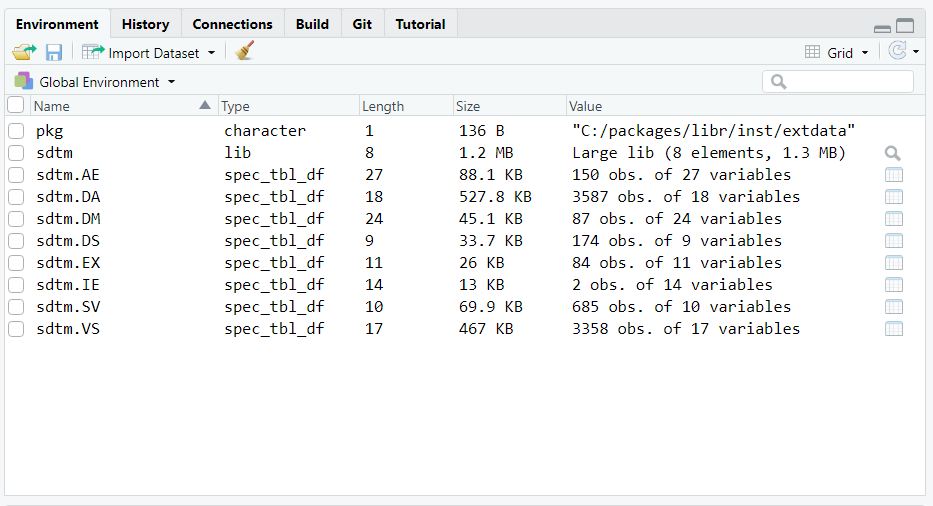
At this point, you can work with your data very much the same way as you would in SAS®. You can pass these datasets into statistical functions, or manipulate them with dplyr functions. Note that you can also work with individual variables on the datasets using dollar sign (“$”) syntax.
# Get total number of records
nrow(sdtm.DM)
# [1] 87

# Get frequency counts for each arm
table(sdtm.DM$ARM)
# ARM A          ARM B          ARM C          ARM D SCREEN FAILURE
# 20             21             21             23              2
The datasets will be available in the workspace for the length of
your session. If you wish to unload them from the workspace, call the
lib_unload() function. See the lib_load() and
lib_unload() documentation for additional information on
these functions.
To see more examples of the libr data management functions, refer to the articles on Basic Library Operations and Library Management.
The dictionary() Function
Once you have a library defined, you may want to examine the column
attributes for the datasets in that library. Examining those column
attributes can be accomplished with the dictionary()
function. The dictionary() function returns a tibble of
information about the data in the library.
Continuing from the example above, let’s look at the dictionary for the ‘sdtm’ library created previously.
dictionary(sdtm)
# # A tibble: 130 x 10
#    Name  Column  Class     Label Description Format Width Justify  Rows   NAs
#    <chr> <chr>   <chr>     <chr> <chr>       <lgl>  <int> <chr>   <int> <int>
#  1 AE    STUDYID character NA    NA          NA         3 NA        150     0
#  2 AE    DOMAIN  character NA    NA          NA         2 NA        150     0
#  3 AE    USUBJID character NA    NA          NA        10 NA        150     0
#  4 AE    AESEQ   numeric   NA    NA          NA        NA NA        150     0
#  5 AE    AETERM  character NA    NA          NA        72 NA        150     0
#  6 AE    AELLT   logical   NA    NA          NA        NA NA        150   150
#  7 AE    AELLTCD logical   NA    NA          NA        NA NA        150   150
#  8 AE    AEDECOD character NA    NA          NA        43 NA        150     0
#  9 AE    AEPTCD  numeric   NA    NA          NA        NA NA        150     0
# 10 AE    AEHLT   character NA    NA          NA        63 NA        150     0
# # ... with 120 more rows
The resulting dictionary table shows the name of the dataset, the
column name, and some interesting attributes related to each column. As
you can see, the libr dictionary table is overall quite
similar to a SAS® dictionary table. See the dictionary()
function documentation for more information.
The datastep() Function
People with experience in SAS® software know that it is sometimes advantageous to process row-by-row. In SAS®, row-by-row processing done with a data step. The data step is one of the most fundamental operations when working in SAS®.
The libr package offers a datastep()
function that simulates this style of row-by-row processing. The
function includes several of the most basic parameters available to the
SAS® datastep: keep, drop, rename, retain, and by. Here is a simple
example, again using the data from the library already defined
above:
age_groups <- datastep(sdtm.DM,
                       keep = c("USUBJID", "AGE", "AGEG"), {

                         if (AGE >= 18 & AGE <= 29)
                           AGEG <- "18 to 29"
                         else if (AGE >= 30 & AGE <= 44)
                           AGEG <- "30 to 44"
                         else if (AGE >= 45 & AGE <= 59)
                           AGEG <- "45 to 59"
                         else
                           AGEG <- "60+"

                       })
age_groups
# # A tibble: 87 x 3
#    USUBJID      AGE AGEG
#    <chr>      <dbl> <chr>
#  1 ABC-01-049    39 30 to 44
#  2 ABC-01-050    47 45 to 59
#  3 ABC-01-051    34 30 to 44
#  4 ABC-01-052    45 45 to 59
#  5 ABC-01-053    26 18 to 29
#  6 ABC-01-054    44 30 to 44
#  7 ABC-01-055    47 45 to 59
#  8 ABC-01-056    31 30 to 44
#  9 ABC-01-113    74 60+
# 10 ABC-01-114    72 60+
# # ... with 77 more rows
Notice that the datastep() function kept only those
variables specified on the keep parameter. The data step
itself is passed within the curly braces. You can put any number of
conditional statements and assignments inside the curly braces, just
like a SAS® data step. Also like a SAS® data step, you do not need to
‘declare’ new variables. Any name not identified as an R function name
is assumed to be a new variable, and will be created automatically on
the input data.
The datastep function also supports “first.” and “last.”
functionality through use of the by parameter. See
additional examples on the datastep() help page and in the
data step article.