Program
The previous examples in the libr documentation were intentionally simplified to focus on the workings of a particular function. It is helpful, however, to also view libr functions in the context of a complete program. The following example shows a complete program. The example illustrates how libr functions work together, and interact with tidyverse and sassy functions to create a report.
The data for this example has been included in the
libr package as an external data file. It may be
accessed using the system.file() function as shown below,
or downloaded directly from the libr GitHub site here
library(tidyverse)
library(sassy)
# Prepare Log -------------------------------------------------------------
options("logr.autolog" = TRUE,
"logr.notes" = FALSE)
# Get temp location for log and report output
tmp <- tempdir()
# Open log
lf <- log_open(file.path(tmp, "example1.log"))
# Load and Prepare Data ---------------------------------------------------
sep("Prepare Data")
# Get path to sample data
pkg <- system.file("extdata", package = "libr")
# Define data library
libname(sdtm, pkg, "csv", quiet = TRUE)
# Prepare data
dm_mod <- sdtm$DM |>
select(USUBJID, SEX, AGE, ARM) |>
filter(ARM != "SCREEN FAILURE") |>
datastep({
if (AGE >= 18 & AGE <= 24)
AGECAT = "18 to 24"
else if (AGE >= 25 & AGE <= 44)
AGECAT = "25 to 44"
else if (AGE >= 45 & AGE <= 64)
AGECAT <- "45 to 64"
else if (AGE >= 65)
AGECAT <- ">= 65"
}) |> put()
put("Get population counts")
arm_pop <- count(dm_mod, ARM) |> put()
sex_pop <- count(dm_mod, SEX) |> put()
agecat_pop <- count(dm_mod, AGECAT) |> put()
# Convert agecat to factor so rows will sort correctly
agecat_pop$AGECAT <- factor(agecat_pop$AGECAT, levels = c("18 to 24",
"25 to 44",
"45 to 64",
">= 65"))
# Sort agecat
agecat_pop <- agecat_pop |> arrange(AGECAT)
# Create Plots ------------------------------------------------------------
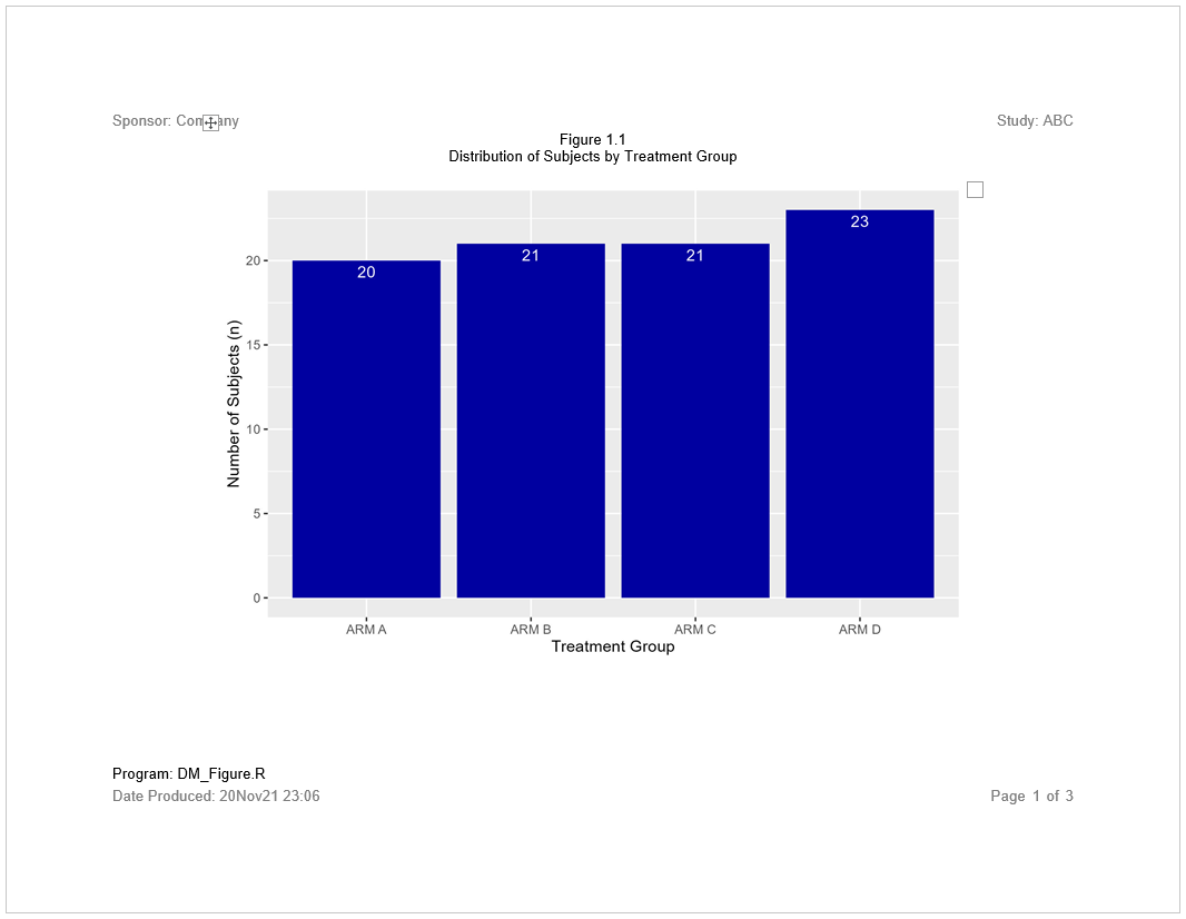
plt1 <- ggplot(data = arm_pop, aes(x = ARM, y = n)) +
geom_col(fill = "#0000A0") +
geom_text(aes(label = n), vjust = 1.5, colour = "white") +
labs(x = "Treatment Group", y = "Number of Subjects (n)")
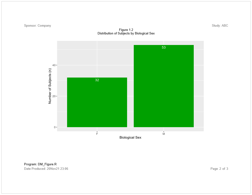
plt2 <- ggplot(data = sex_pop, aes(x = SEX, y = n)) +
geom_col(fill = "#00A000") +
geom_text(aes(label = n), vjust = 1.5, colour = "white") +
labs(x = "Biological Sex", y = "Number of Subjects (n)")
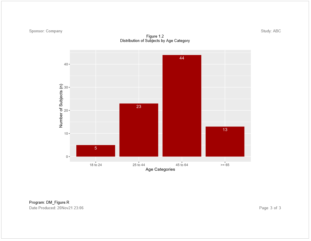
plt3 <- ggplot(data = agecat_pop, aes(x = AGECAT, y = n)) +
geom_col(fill = "#A00000") +
geom_text(aes(label = n), vjust = 1.5, colour = "white") +
labs(x = "Age Categories", y = "Number of Subjects (n)")
# Report ------------------------------------------------------------------
sep("Create and print report")
page1 <- create_plot(plt1, 4.5, 7) |>
titles("Figure 1.1", "Distribution of Subjects by Treatment Group")
page2 <- create_plot(plt2, 4.5, 7) |>
titles("Figure 1.2", "Distribution of Subjects by Biological Sex")
page3 <- create_plot(plt3, 4.5, 7) |>
titles("Figure 1.2", "Distribution of Subjects by Age Category")
rpt <- create_report(file.path(tmp, "./output/example1.rtf"), output_type = "RTF",
font = "Arial") |>
set_margins(top = 1, bottom = 1) |>
page_header("Sponsor: Company", "Study: ABC") |>
add_content(page1) |>
add_content(page2) |>
add_content(page3) |>
footnotes("Program: DM_Figure.R") |>
page_footer(paste0("Date Produced: ", fapply(Sys.time(), "%d%b%y %H:%M")),
right = "Page [pg] of [tpg]")
res <- write_report(rpt)
# Clean Up ----------------------------------------------------------------
sep("Clean Up")
# Close log
log_close()
# View log
# file.show(lf)
# View report
# file.show(res$file_path)Log
Here is the log from the above program:
=========================================================================
Log Path: C:/Users/dbosa/AppData/Local/Temp/RtmpwLpEIV/log/example1.log
Program Path: C:\packages\Testing\libr_example1.R
Working Directory: C:/packages/Testing
User Name: dbosa
R Version: 4.1.2 (2021-11-01)
Machine: SOCRATES x86-64
Operating System: Windows 10 x64 build 19041
Base Packages: stats graphics grDevices utils datasets methods base
Other Packages: tidylog_1.0.2 reporter_1.2.6 libr_1.2.1 fmtr_1.5.4 logr_1.2.7
                sassy_1.0.5 forcats_0.5.1 stringr_1.4.0 dplyr_1.0.7 purrr_0.3.4
                readr_2.0.2 tidyr_1.1.4 tibble_3.1.5 ggplot2_3.3.5 tidyverse_1.3.1
Log Start Time: 2021-11-20 23:06:50
=========================================================================

=========================================================================
Prepare Data
=========================================================================

# library 'sdtm': 8 items
- attributes: csv not loaded
- path: C:/Users/dbosa/Documents/R/win-library/4.1/libr/extdata
- items:
  Name Extension Rows Cols     Size        LastModified
1   AE       csv  150   27  88.3 Kb 2021-10-08 15:02:15
2   DA       csv 3587   18 528.1 Kb 2021-10-08 15:02:15
3   DM       csv   87   24  45.4 Kb 2021-10-08 15:02:15
4   DS       csv  174    9  33.9 Kb 2021-10-08 15:02:15
5   EX       csv   84   11  26.2 Kb 2021-10-08 15:02:15
6   IE       csv    2   14  13.2 Kb 2021-10-08 15:02:15
7   SV       csv  685   10  70.2 Kb 2021-10-08 15:02:15
8   VS       csv 3358   17 467.3 Kb 2021-10-08 15:02:15

lib_load: library 'sdtm' loaded

select: dropped 20 variables (STUDYID, DOMAIN, SUBJID, RFSTDTC, RFENDTC, <U+0085>)

filter: removed 2 rows (2%), 85 rows remaining

datastep: columns increased from 4 to 5

# A tibble: 85 x 5
   USUBJID    SEX     AGE ARM   AGECAT
   <chr>      <chr> <dbl> <chr> <chr>
 1 ABC-01-049 M        39 ARM D 25 to 44
 2 ABC-01-050 M        47 ARM B 45 to 64
 3 ABC-01-051 M        34 ARM A 25 to 44
 4 ABC-01-052 F        45 ARM C 45 to 64
 5 ABC-01-053 F        26 ARM B 25 to 44
 6 ABC-01-054 M        44 ARM D 25 to 44
 7 ABC-01-055 F        47 ARM C 45 to 64
 8 ABC-01-056 M        31 ARM A 25 to 44
 9 ABC-01-113 M        74 ARM D >= 65
10 ABC-01-114 F        72 ARM B >= 65
# ... with 75 more rows

Get population counts

count: now 4 rows and 2 columns, ungrouped

# A tibble: 4 x 2
  ARM       n
  <chr> <int>
1 ARM A    20
2 ARM B    21
3 ARM C    21
4 ARM D    23

count: now 2 rows and 2 columns, ungrouped

# A tibble: 2 x 2
  SEX       n
  <chr> <int>
1 F        32
2 M        53

count: now 4 rows and 2 columns, ungrouped

# A tibble: 4 x 2
  AGECAT       n
  <chr>    <int>
1 >= 65       13
2 18 to 24     5
3 25 to 44    23
4 45 to 64    44

=========================================================================
Create and print report
=========================================================================

# A report specification: 3 pages
- file_path: 'C:\Users\dbosa\AppData\Local\Temp\RtmpwLpEIV/./output/example1.rtf'
- output_type: RTF
- units: inches
- orientation: landscape
- margins: top 1 bottom 1 left 1 right 1
- line size/count: 9/40
- page_header: left=Sponsor: Company right=Study: ABC
- footnote 1: 'Program: DM_Figure.R'
- page_footer: left=Date Produced: 20Nov21 23:06 center= right=Page [pg] of [tpg]
- content:
# A plot specification:
- data: 4 rows, 2 cols
- layers: 2
- height: 4.5
- width: 7
- title 1: 'Figure 1.1'
- title 2: 'Distribution of Subjects by Treatment Group'
# A plot specification:
- data: 2 rows, 2 cols
- layers: 2
- height: 4.5
- width: 7
- title 1: 'Figure 1.2'
- title 2: 'Distribution of Subjects by Biological Sex'
# A plot specification:
- data: 4 rows, 2 cols
- layers: 2
- height: 4.5
- width: 7
- title 1: 'Figure 1.2'
- title 2: 'Distribution of Subjects by Age Category'

=========================================================================
Clean Up
=========================================================================

lib_sync: synchronized data in library 'sdtm'

lib_unload: library 'sdtm' unloaded

=========================================================================
Log End Time: 2021-11-20 23:06:57
Log Elapsed Time: 0 00:00:07
=========================================================================